In probability theory and statistics, the Bernoulli distribution, named after Swiss mathematician Jacob Bernoulli, is the discrete probability distribution of a random variable which takes the value 1 with probability p and the value 0 with probability q=1-p, that is, the probability distribution of any single experiment that asks a yes–no question; the question results in a boolean-valued outcome, a single bit of information whose value is success/yes/true/one with probability p and failure/no/false/zero with probability q. It can be used to represent a (possibly biased) coin toss where 1 and 0 would represent "heads" and "tails" (or vice versa), respectively, and p would be the probability of the coin landing on heads or tails, respectively. In particular, unfair coins would have p ≠ 1/2.

Probability Mass Function
The binomial distribution with parameters n and p is the discrete probability distribution of the number of successes in a sequence of n independent experiments, each asking a yes–no question, and each with its own boolean-valued outcome: a random variable containing single bit of information: success/yes/true/one (with probability p) or failure/no/false/zero (with probability q = 1 − p). A single success/failure experiment is also called a Bernoulli trial or Bernoulli experiment and a sequence of outcomes is called a Bernoulli process; for a single trial, i.e., n = 1, the binomial distribution is a Bernoulli distribution. The binomial distribution is the basis for the popular binomial test of statistical significance.
Is a discrete probability distribution of the number of successes in a sequence of independent and identically distributed Bernoulli trials before a specified (non-random) number of failures (denoted r) occurs.
Different texts adopt slightly different definitions for the negative binomial distribution. They can be distinguished by whether the support starts at k = 0 or at k = r, whether p denotes the probability of a success or of a failure, and whether r represents success or failure, so it is crucial to identify the specific parametrization used in any given text.

The orange line represents the mean, which is equal to 10 in each of these plots; the green line shows the standard deviation.
Suppose there is a sequence of independent Bernoulli trials . Thus, each trial has two potential outcomes called "success" and "failure". In each trial the probability of success is p and of failure is (1 − p). We are observing this sequence until a predefined number r of failures has occurred. Then the random number of successes we have seen, X, will have the negative binomial (or Pascal) distribution:

In probability theory and statistics, the geometric distribution is either of two discrete probability distributions:
- The probability distribution of the number X of Bernoulli trials needed to get one success, supported on the set { 1, 2, 3, ... }
- The probability distribution of the number Y = X − 1 of failures before the first success, supported on the set { 0, 1, 2, 3, ... }

Probability Mass Function
The geometric distribution gives the probability that the first occurrence of success requires k independent trials, each with success probability p. If the probability of success on each trial is p, then the probability that the kth trial (out of k trials) is the first success is:

for k = 1, 2, 3, ....
The above form of the geometric distribution is used for modeling the number of trials up to and including the first success. By contrast, the following form of the geometric distribution is used for modeling the number of failures until the first success:

for k = 0, 1, 2, 3, ....
In either case, the sequence of probabilities is a geometric sequence.
Is a discrete probability distribution that describes the probability of k successes (random draws for which the object drawn has a specified feature) in n draws, without replacement, from a finite population of size N that contains exactly K objects with that feature, wherein each draw is either a success or a failure.
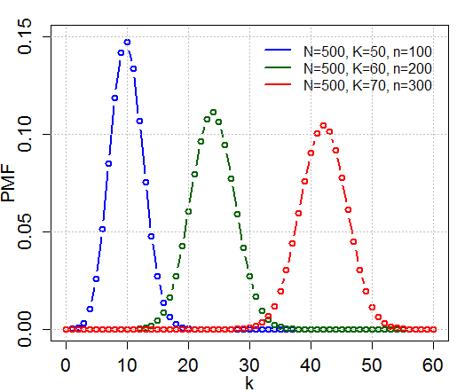
Probability Mass Function
The following conditions characterize the hypergeometric distribution:
- The result of each draw (the elements of the population being sampled) can be classified into one of two mutually exclusive categories (e.g. Pass/Fail or Employed/Unemployed).
- The probability of a success changes on each draw, as each draw decreases the population ( sampling without replacement from a finite population).

where:
- N is the population size
- K is the number of success states in the population
- n is the number of draws (i.e. quantity drawn in each trial)
- k is the number of observed successes
is a binomial coefficient.
Is a family of discrete probability distributions on a finite support of non-negative integers arising when the probability of success in each of a fixed or known number of Bernoulli trials is either unknown or random.

Probability Mass Function
The Beta distribution is a conjugate distribution of the binomial distribution. This fact leads to an analytically tractable compound distribution where one can think of the p parameter in the binomial distribution as being randomly drawn from a beta distribution. Namely, if:

then

where Bin(n,p) stands for the binomial distribution, and where p is a random variable with a beta distribution.
The predictive distribution is given by:
